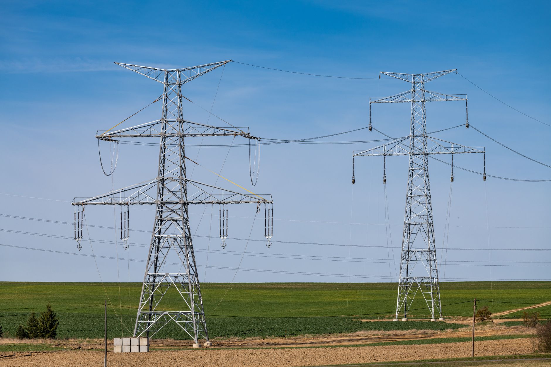
On a hot afternoon, a transmission line carrying power toward a load centre approaches its thermal rating. The flow cannot increase without risking conductor damage or a clearance violation, so the system operator changes dispatch: cheaper generation on one side of the line is held back, and more expensive generation on the other side serves the load. This is what grid congestion causes in its most ordinary form: a price difference between two locations that are electrically close, a spread that is the market’s expression of a physical limit.
Congestion has become a recurring feature of systems where generation resources develop far from load centres and move in patterns the network was not originally built around. Wind and solar output shifts with weather; demand shifts with electrification and new industrial loads. The same physical limits that once affected only a few corridors now interact with more dispersed generation and more variable demand.
This article traces congestion from cause to consequence: a constraint on one corridor, the node-to-node price spread it produces, the curtailment and redispatch decisions that follow, and the investment signal that persists across many hours. The aim is to make the links between physics, market prices, and planning decisions easier to read, without arguing whether congestion is good or bad.
Market participants read congestion signals in several distinct ways. A spread that appears in day-ahead prices may reflect expected scarcity; the same spread in real time often reflects a binding physical limit. Analysts compare those two pictures to see whether the constraint was anticipated or emerged as weather, load, or unit availability changed.
Transmission planners, meanwhile, work on much slower timelines. A corridor that binds only a few hours a year can be hard to justify against alternatives such as local generation, batteries, or demand response. Congestion therefore sits at the intersection of instantaneous physics and long-lived investment decisions, and professionals across market and planning teams need a common language for it.
The Physical Limits Behind Congestion
Congestion begins with a basic property of alternating-current networks: power flows along all available paths in inverse proportion to impedance, not along the contractual route a trader has chosen. A line can be loaded by a transaction that nominally occurs hundreds of kilometres away. That loop flow can make a line that appears unrelated to a transaction into a constraint across the wider system.
Thermal limits are a common source. A transmission line can carry current only until conductor heating causes it to sag beyond its clearance limit or degrade the material. That limit is not fixed. It depends on ambient temperature, wind speed, and how long the line has already been running near its rating. A line can carry more on a cold, windy night than on a still, hot afternoon because wind removes heat from the conductor. Operators therefore use seasonal ratings, and in some cases dynamic line ratings, rather than a single permanent value.
Voltage and stability limits are less obvious but equally real. When a line carries high reactive power or a long transfer over a single corridor, voltage can fall below acceptable levels. In some systems, the binding limit is not current but the risk that a fault would separate the corridor and cause instability. These constraints can curtail power even when a line is not thermally overloaded.
What all of these have in common is that the network’s ability to move power is finite. Thermal ratings, voltage limits and stability margins describe different mechanisms, but they produce the same practical outcome: a maximum transfer the system can carry across a given interface at a given moment. When demand or generation patterns push transfers against that limit, the system is congested, and the market effects that follow all begin from that physical condition.
From a Binding Constraint to a Price Spread
Where markets use locational pricing, each node or zone has its own price, and congestion appears as the difference between them. If a low-cost generator in a surplus region cannot move additional power to a high-demand region because a line between them is at its limit, the market operator must meet demand with a higher-cost unit on the demand side. That unit’s offer sets the local price. The spread between the two locations is a shadow price of transmission scarcity: it approximates the marginal cost of relieving the constraint, or the extra system cost of moving one more megawatt across the line rather than generating locally.
In nodal markets such as ERCOT and PJM’s day-ahead and real-time markets, these differences appear continuously. They are the expected output of the pricing system. A trader may buy transmission rights or locate generation to capture the spread, but the underlying signal remains the same: the network could not carry enough power from the low-price side to the high-price side.
In ERCOT, a common pattern involves wind generation in West Texas and load in Dallas and Houston. When the transmission paths out of West Texas bind, prices in the west can fall while prices in load centres rise. A similar separation appears in California during spring midday hours when solar output exceeds local demand and export paths are full, often contributing to the curtailment decisions discussed in the article on renewable curtailment.
Real-Time Redispatch and Operational Choices
Market operators do not wait for lines to overload. Security-constrained economic dispatch includes network limits in the optimisation. When the least-cost dispatch would exceed a line’s rating, the operator moves to the next least-cost combination that keeps flows within limits. That process is redispatch, and it is why a constrained hour can include out-of-merit generation: units run because of where they are, not only because of what they cost.
Some units are kept available not because they are cheap, but because their location supports voltage, stability, or local reserves. A grid operator may contract such a unit as reliability must-run, paying it separately to remain available even when its energy would not clear in a simple market. This is an operational response to a congestion-related reliability risk, rather than a market distortion.
Day-ahead markets clear units against forecasted constraints, while real-time redispatch adjusts for conditions that differ from the forecast. The two markets can therefore show different congestion patterns. Analysts often compare day-ahead and real-time spreads to see whether a constraint was anticipated or emerged as weather, load, or unit availability changed. The day-ahead signal tells you what the market expected; the real-time signal tells you what the constraint actually required.
Curtailment as an Operational Outcome
When generation output exceeds what the local network can move, curtailment is a standard operational tool. The operator instructs wind or solar plants to reduce output, often because a transmission corridor is at its limit and demand cannot absorb the surplus. In markets with high renewable penetration, this can happen in specific seasons rather than uniformly across the year.
California’s spring midday hours provide a concrete pattern. Solar output rises while demand remains moderate, and transmission paths out of the surplus zones are often full. The result is curtailment, along with low or negative prices in the constrained region. Whether that curtailment is best understood as a market failure or a rational operational choice is a separate question, examined in the article on renewable curtailment.
Analysts distinguish between economic curtailment, where a plant’s bid is above the local price, and operational curtailment, where the plant receives an instruction regardless of price. Congestion-driven curtailment is usually the second type: the resource is available and cheap, but the network cannot move its output. That distinction helps explain why adding storage or load in the surplus zone can reduce curtailment even without building a new transmission line.
Who Bears the Cost of a Congested Corridor
Congestion creates price differences, and those differences transfer value between buyers and sellers. A load in a constrained zone often pays a higher locational price than a load on the other side of the constraint. A generator in the surplus zone may receive less, while a generator in the deficit zone may receive more. The total additional cost to consumers in constrained hours is often described as congestion cost, and it can be substantial in markets where a few corridors bind frequently.
In regions with financial transmission rights, some of that congestion revenue can be allocated to rights holders as a hedge. Where such rights exist, a participant who expects a corridor to be congested can buy a right that receives a payment when the spread appears. The design aims to turn a volatile price difference into something that can be priced in advance, but it does not remove the underlying physical constraint. A fuller treatment appears in the article on the hidden cost of grid congestion.
Congestion cost is not the same as the cost of fixing congestion. A new transmission line may reduce price spreads but involves substantial capital and long lead times. A battery, a demand response programme, or a gas plant placed on the load side can reduce constraints at smaller scale. The comparison between paying congestion cost and investing to remove it is a central planning question.
Historical Context: A Network Built for a Different Flow Pattern
Existing transmission networks were largely planned when generation came from large thermal plants close to load centres or fuel supply. Interconnection rules, grid codes, and market designs inherited that assumption: power flowed predictably from a few plants toward cities and industrial regions. Congestion existed, but it was often confined to a limited number of corridors and managed with established operating procedures.
The current system is different. Wind and solar resources are built where the resource is strongest, not where the load is. New gas plants may be located near gas infrastructure rather than at the centre of load pockets. Rooftop solar, electrified transport, and data centre demand further shift the spatial pattern. Consequently, corridors that rarely bound in the past may now bind during particular weather conditions or seasons.
This legacy shape matters because it affects how easily the network can adapt. A line designed to connect a coal plant to a metropolis may still serve that load, but it was not sized to carry the output of distant wind farms in the opposite direction of historical flow. That mismatch helps explain why congestion appears in different places than older planning studies anticipated.
The Transmission Investment Feedback Loop
A persistent node-to-node spread is, among other things, an investment signal. If the same corridor binds across many hours, the value of additional capacity may be high. But transmission planning is slow and lumpy: a new line changes flows across a wide area, may create new constraints elsewhere, and its cost is recovered through rates or market charges in ways that depend on jurisdiction, market design and regulatory framework. The link between a market signal and a completed project is therefore never automatic.
Analysts tend to consider not only the size of a spread but its duration, frequency and shape. A few extreme hours during a heat wave may justify a small, targeted solution rather than a major line. A spread that persists through most days across seasons suggests a deeper mismatch between generation locations and load. The same logic appears when planners choose between transmission, storage, demand response, or local generation as the least-cost way to reduce constraints.
This investment question is tied to the cost discussion in the article on the hidden cost of grid congestion. A recurring constraint can create substantial total congestion cost, but the business case for a line depends on who receives the benefits and who pays. In some markets, cost allocation rules make regional projects harder to approve; in others, anticipatory planning frameworks are more developed. That institutional variation is one reason the same physical congestion can lead to different investment outcomes.
How Analysts Read the Signals
Different market participants read congestion differently because their risks differ. A generator evaluates congestion as a locational price risk: its output may be worth less when a nearby corridor binds. A load-serving entity sees the same spread as an input cost, and may hedge with transmission rights or contracts tied to a specific node. A trader focuses on the difference between day-ahead and real-time spreads, which can reflect how well the market anticipated the constraint.
Analysts often separate the signal into two parts. A day-ahead spread indicates what the market expected before conditions were fully known; a real-time spread indicates what the constraint actually required. Comparing them can reveal forecast error, weather sensitivity, or unplanned unit outages. It can also show when a constraint is structural rather than occasional.
Some signals are indirect. Low or negative prices in a region with abundant renewable output, alongside high prices in a neighbouring region, point toward a transmission limit rather than a lack of demand. Curtailment records provide similar evidence: if a plant is cut off while local prices are very low, the constraint is likely to be network- or stability-related rather than a simple market price signal. The article on renewable curtailment works through that distinction in more detail.
These signals do not provide a simple ranking. A high spread does not, by itself, mean a line should be built; it means the system is paying to live with a physical limit. Reading congestion well requires combining the price signal with operational records, weather data, and a clear view of who benefits from alternative fixes.
Where to Go Next
Three ideas from this article are worth keeping in view. First, congestion starts with a physical limit — usually thermal, voltage, or stability — and the market’s role is to reveal that limit through locational prices. Second, the node-to-node price spread is the shadow price of that limit, showing the marginal value of more transfer capability during constrained hours. Third, a spread is only part of the story. Analysts also look at how often it appears, whether it was anticipated, and what alternatives exist before concluding that a new line is the right answer.
If the financial consequences are what brought you here, the article on the hidden cost of grid congestion explains where those costs land and how they are hedged in more detail. If the operational choice to switch off available generation is the part that interests you, the piece on renewable curtailment works through the difference between market failure and rational operations.
The common thread across these pieces is that congestion is a physical fact with a market expression. Thermal limits, voltage constraints and the switching state of the network decide where power can flow; dispatch, prices and hedging arrangements decide who carries the cost of the difference. Understanding one without the other leads to incomplete decisions — whether the next step is an investment, a hedge, or a new operating practice.
References
- International Energy Agency — World Energy Outlook 2025. Provided context on electricity demand growth and grid investment needs underlying congestion pressures.
- International Energy Agency — Electricity 2025. Provided background on system flexibility and grid constraints in markets with rising renewable output.
- North American Electric Reliability Corporation — Long-Term Reliability Assessment. Informed discussion of transmission constraints, operational margins, and reliability-driven measures such as reliability must-run contracts.